RooFit

The RooFit library provides a set of tools for modeling the expected distribution of events. in physical analysis. Models can be used to perform the most believable fitting, creating graphs and applying the Monte Carlo method for various studies

RooFit is an extension of ROOT, but is not installed by default with it. On the LIT cluster hybrilit.jinr.ru version of ROOT6 compiled with RooFit. ROOT5 on this cluster does not allow use RooFit.

The main functionality of RooFit is the ability to simulate ‘event data’ distributions, where each event is a discrete event in time, and has one or more measurable observables associated with it. Experiments of this kind lead to data sets obeying Poisson statistics (or binomial distribution).

The natural modeling language for such distributions is a probability density function F (x, p), describing the probability density of the distribution of the observed x as a function depending on the parameter p. In probability theory, the probability density function (P.d.f) or the density of continuous random values is a function whose value for any given sample (or point) in space samples (a set of possible values taken by a random variable) can be interpreted as providing a relative probability that the value of the random variable will be equal to this sample. The defining properties of the probability density function: normalization by one over all observables and positive certainty also provide important design benefits. Density functions probabilities are easily added; it is possible to construct multidimensional P.d.f from one-dimensional with intuitive clear description of the correlations between the observed. Also, these functions allow universal application of the Monte Carlo method.

RooFit uses a special method when converting the components of mathematical data models to C++ objects; instead of aiming at the monolithic object that describes the data object, Each mathematical symbol is represented by a separate object. All RooFit models always consist of multiple objects.

For example, the Gauss probability density function consists typically of four objects: three objects, representing the observed value, the average value and the Sigma parameter, and one object, representing the Gauss probability density function. That is, to be able to work with probability density function, it is necessary to create all four objects sequentially. Similarly, the construction of operations such as addition, multiplication, integration - represented by separate objects. Such a universal modeling language is good. for models of arbitrary complexity. A list of all classes of the RooFit library with their detailed description can be found by link . RooFit makes no difference between observables and parameters. Both those and others are implemented using RooRealVar class. We give a general view of the constructors of the RooRealVar and RooGaussian classes:

RooRealVar::RooRealVar(const char *name, const char *title, Double_t value, Double_t minValue, Double_t maxValue,

const char *unit)

RooGaussian (const char *name, const char *title, RooAbsReal &_x, RooAbsReal &_mean, RooAbsReal &_sigma)

Here name is the variable (signal) name, the unique identifier of the object, and title is the variable title. (signal) with a more detailed description of the object, value - the value value, minValue - the minimum value, maxValue - the minimum value, unit - the unit of magnitude (optional value), x is the observed value, mean is the mean, sigma is the standard deviation.

An object of class RooAddPdf is an effective implementation of the sum p.d.f in the form

c1 * PDF1 + c2 * PDF2 + ... сп * PDFn or

c1 * PDF1 + c2 * PDF2 + ... (1-sum (c1 ... сп-1)) * PDFn

The first form is for extended likelihood, where the expected number of events is Σici. The coefficients c_i can be either specified explicitly or, if all components support extended plausibility, they can be calculated as the contribution of each p.d.f to the total number of expected events. In the second form, the sum of the coefficients is equal to one, and the coefficient of the last p.d.f calculated from this condition. It is also possible to parameterize coefficients recursively

c1 * PDF1 + (1-с1) (c2 * PDF2 + (1-c2) * (c3 * PDF3 + ....))

In this form, the sum of the coefficients is always less than 1 for all possible values of individual coefficients between 0 and 1. RooAddPdf believes that each component is already normalized and does not perform any normalization, except calculate the corresponding last coefficient c_n, if required. Condition (mandatory) for this addition, each PDF_i is independent of each coefficient_i.

Consider an example of how to build a one-dimensional probability density function with two components: Gauss signal and background. Working with the RooFit library is also possible through the CINT interpreter and running macros. In both cases, it is recommended to turn to space at the beginning. RooFit names to be able to use predefined constants and other various identifiers (names of types, functions, variables, etc.)

root[0] using namespace RooFit;

root[1] RooRealVar mes("mes","m_{ES} (GeV)",5.20,5.30)

root[2] RooRealVar sigmean("sigmean","B^{#pm} mass",5.28,5.20,5.30)

root[3] RooRealVar sigwidth("sigwidth","B^{#pm} width",0.0027,0.001,1.)

root[4] RooGaussian Signal("Signal","signal PDF",mes,sigmean,sigwidth)

root[5] RooRealVar argpar("argpar","argus shape parameter",-20.0,-100.,-1.)

root[6] RooArgusBG background("background","Argus PDF",mes,RooConst(5.291),argpar)

root[7] RooRealVar nsig("nsig","#signal events",200,0.,10000)

root[8] RooRealVar nbkg("nbkg","#background events",800,0.,10000)

root[9] RooAddPdf model("model","g+a",RooArgList(signal,background),RooArgList(nsig,nbkg))

root[10] RooDataSet *data = model.generate(mes,2000)

root[11] model.fitTo(*data)

root[12] RooPlot* mesframe = mes.frame()

root[13] data->plotOn(mesframe)

root[14] model.plotOn(mesframe)

root[15] mesframe->Draw()

Comments for example:

• [0]-connect the RooFit namespace. (Note the need for a semicolon in this command).

• [1]-we define the observed value.

• [2-3]-define the signal parameters.

• [4]-we construct the signal (in the name of the variable we use uppercase letter S to avoid identity with file name signal.h in standard C ++ 11.

• [5]-we define the background parameters.

• [6]-we design the background.

• [7-9]-we construct the model (signal + background).

• [10]-generate 2000 events.

• [11]-perform fitting.

• [12-15]-draw a combined p.d.f and data played on it. The object of the RooPlot class is an empty frame, capable of holding something (RooDataSet; PDF projections and general projections of real functions; any ROOT object: arrows, text boxes, ... - which can be drawn) depending on its variable.

As a result of the actions above, we get the following picture.

To get mean and sigma values, use the Print method. In this case:

root[16] sigmean.Print()

root[17] sigwidth.Print()

You can also add the p.d.f parameter field and the statistics field to the screen:

root[18] model.paramOn(mesframe,data)

root[19] data.statOn(mesframe)

root[20] mesframe->Draw()

Convolution example of two probability density functions

The first example shows the use of the addition operator of two p.d.f. RooAddPdf for compiling a common p.d.f. It is also possible to construct a convolution p.d.f.th using the convolution operator implemented in the class RooFFTConvPdfF.

root[0] using namespace RooFit ;

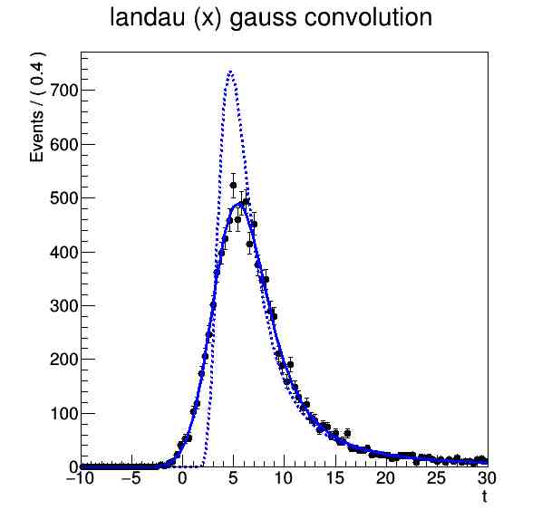
We construct the observed value of t [1], the average value and the standard deviation for the two distributions Landau and Gauss [2-5]. We build the distributions themselves [6-7]. We construct a convolution of Landau and Gauss. We make a sample of 10,000 events, we fit the data. We build a graph on which we present: the probability density function of the resulting convolution (solid line), the data drawn by this function (markers) and p.d.f. Landau (dashed line).

root[1] RooRealVar t("t","t",-10,30)

root[2] RooRealVar ml("ml","mean landau",5.,-20,20)

root[3] RooRealVar sl("sl","sigma landau",1,0.1,10)

root[4] RooRealVar mg("mg","mean gauss",0)

root[5] RooRealVar sg("sg","sigma gauss",2,0.1,10)

root[6] RooLandau landau("lx","lx",t,ml,sl)

root[7] RooGaussian gauss("gauss","gauss",t,mg,sg)

// Set #bins to be used for FFT sampling to 10000

root[8] t.setBins(10000,"cache") ;

root[9] RooFFTConvPdf lxg("lxg","landau (X) gauss",t,landau,gauss) ;

root[10] RooDataSet* data = lxg.generate(t,10000) ;

root[11] lxg.fitTo(*data) ;

root[12] RooPlot* frame = t.frame(Title("landau (x) gauss convolution")) ;

root[13] data->plotOn(frame) ;

root[14] lxg.plotOn(frame) ;

root[15] landau.plotOn(frame,LineStyle(kDashed)) ;

root[16] new TCanvas("convolution","convolution",600,600) ;

root[17] gPad->SetLeftMargin(0.15) ;

root[18] frame->GetYaxis()->SetTitleOffset(1.4) ;

root[19] frame->Draw() ;

An example of a multidimensional p.d.f.

You can also construct a multidimensional probability density function and its projection on the x and y axes.

Create observables:

RooRealVar x("x","x",-5,5) ;

RooRealVar y("y","y",-5,5) ;

Create parameters and function f (y) = a0 + a1 * y

RooRealVar a0("a0","a0",-0.5,-5,5) ;

RooRealVar a1("a1","a1",-0.5,-1,1) ;

RooPolyVar fy("fy","fy",y,RooArgSet(a0,a1)) ;

Create Gauss (x, f (y), s)

RooRealVar sigma("sigma","width of gaussian",0.5) ;

RooGaussian model("model","Gaussian with shifting mean",x,fy,sigma) ;

We generate 10,000 events distributed by this model.

RooDataSet *data = model.generate(RooArgSet(x,y),10000) ;

Create a graph x data distribution and projection of the model on x = Int (dy) model (x, y)

RooPlot* xframe = x.frame() ;

data->plotOn(xframe) ;

model.plotOn(xframe) ;

Create a graph x data distribution and projection of the model on x = Int (dy) model(x,y)

RooPlot* yframe = y.frame() ;

data->plotOn(yframe) ;

model.plotOn(yframe) ;

Create a two-dimensional histogram of x from y

TH1* hh_model = model.createHistogram("hh_model",x,Binning(50),YVar(y,Binning(50))) ;

hh_model->SetLineColor(kBlue) ;

Create a screen and draw graphics

TCanvas *c = new TCanvas("rf301_composition","rf301_composition",1200, 400);

c->Divide(3);

c->cd(1) ; gPad->SetLeftMargin(0.15) ; xframe->GetYaxis()->SetTitleOffset(1.4) ; xframe->Draw() ;

c->cd(2) ; gPad->SetLeftMargin(0.15) ; yframe->GetYaxis()->SetTitleOffset(1.4) ; yframe->Draw() ;

c->cd(3) ; gPad->SetLeftMargin(0.20) ; hh_model->GetZaxis()->SetTitleOffset(2.5) ; hh_model->Draw("surf") ;

The figure below shows a two-dimensional visualization of M (X, Y) and the projections on observable t x and y c data superimposed on them.

Example of working with probability functions and their profile projections

The previous examples have illustrated various techniques for building a probability density function. in RooFit. This example demonstrates various operations that can be applied at the probability level. Given p.d.f and a data set, the probability function can be constructed as

RooAbsReal* nll = pdf.createNLL(data) ;

Likelihood functions behave like normal RooFit functions and can be built in the same way as functions probability density.

RooPlot* frame = myparam.frame() ;

nll->plotOn(frame) ;

Since probability estimation is a potentially time consuming operation, RooFit makes it easier to calculate the probability using parallel multiple processes. This parallelization process is transparent to the user. By requesting parallel computations on 8 processors (on one node), you can build a likelihood function in the following way

RooAbsReal* nll = pdf.createNLL(data,NumCPU(8)) ;

It is also possible by analogy to construct projections of probabilities on different quantities.

RooAbsReal* pll = nll->createProfile(paramOfInterest)

Consider an example of how to construct p.d.f and a data set and compare the probability and probability projection on one of the parameters.

So, create a model and a data set

root[1] RooRealVar x("x","x",-20,20)

root[2] RooRealVar mean("mean","mean of g1 and g2",0,-10,10)

root[3] RooRealVar sigma_g1("sigma_g1","width of g1",3)

root[4] RooGaussian g1("g1","g1",x,mean,sigma_g1)

root[5] RooRealVar sigma_g2("sigma_g2","width of g2",4,3.0,6.0)

root[6] RooGaussian g2("g2","g2",x,mean,sigma_g2)

root[7] RooRealVar frac("frac","frac",0.5,0.0,1.0)

root[8] RooAddPdf model("model","model",RooArgList(g1,g2),frac) // Модель (интенсивные сильные корреляции)

root[9] RooDataSet* data = model.generate(x,1000)

Construct credibility Build Unlimited Likelihood

root[10] RooAbsReal* nll = model.createNLL(*data,NumCPU(2))

Minimizing the likelihood of all parameters before the execution of the schedule

root[11] RooMinimizer(*nll).migrad()

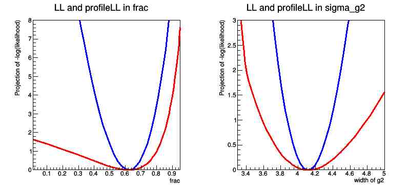
Drawing a frac likelihood sweep

root[12] RooPlot* frame1 = frac.frame(Bins(10),Range(0.01,0.95),Title("LL and profileLL in frac"))

root[13] nll->plotOn(frame1,ShiftToZero())

Drawing a likelihood sweep by sigma_g2

root[14] RooPlot* frame2 = sigma_g2.frame(Bins(10),Range(3.3,5.0),Title("LL and profileLL in sigma_g2"))

root[15] nll->plotOn(frame2,ShiftToZero())

We build the probability projection on frac Profile Profile Likelihood Estimator for Frac minimizes nll w.r.t all float parameters except frac for each rating

root[16] RooAbsReal* pll_frac = nll->createProfile(frac)

Draw a probability projection on frac

root[17] pll_frac->plotOn(frame1,LineColor(kRed))

Adjust frame maximum for visual clarity

root[18] frame1->SetMinimum(0)

root[19] frame1->SetMaximum(3)

We build the probability projection on sigma_g2. The profile probability estimator on nll for sigma_g2 minimizes the nll w.r.t of all floating parameters, except sigma_g2 for each evaluation Draw a probability projection by sigma_g2

root[20] pll_sigmag2->plotOn(frame2,LineColor(kRed))

Adjust frame maximum for visual clarity

root[21] frame2->SetMinimum(0)

root[22] frame2->SetMaximum(3)

Create a screen and draw RooPlots

root[23] Canvas *c = new TCanvas("rf605_profilell","rf605_profilell",800, 400)

root[24] c->Divide(2)

root[25] c->cd(1)

root[26] gPad->SetLeftMargin(0.15)

root[27] frame1->GetYaxis()->SetTitleOffset(1.4)

root[28] frame1->Draw()

root[29] c->cd(2)

root[30] gPad->SetLeftMargin(0.15)

root[31] frame2->GetYaxis()->SetTitleOffset(1.4)

root[32] frame2->Draw()

root[33] delete pll_frac

root[34] delete pll_sigmag2

root[35] delete nll

The resulting graph contains the probabilities and the projection of the probability on the flac parameter, as well as a similar graph for projection on the sigma_g2 parameter.

Training Programs and Documentation

A set of 83 training macros (as well as a link to the User’s Guide) are available in the distribution at $ ROOTSYS/tutorials/roofit. (On hybrilit cluster - at /cvmfs/hybrilit.jinr.ru/sw/root/6.09.02/sl6-gcc49/tutorials/roofit) Detailed documentation of all classes with methods and data members is available on the official ROOT website in .pdf format.